Compile and Build the Model

Compile the Model

#@title Compile model

learning_rate = 1e-3  # students can tune (= 0.001)

model.compile(
    optimizer=keras.optimizers.Adam(learning_rate=learning_rate),
    loss="binary_crossentropy",
    metrics=[
        "accuracy",
        keras.metrics.AUC(name="auc"),
    ],
)

model.compile(...) tells Keras:

• how to update the model (optimizer)
• how to measure errors (loss function)
• which metrics to compute during training/evaluation

It does not start training yet – it just configures the training procedure.

Learning rate

learning_rate = 1e-3  # = 0.001

The learning rate controls how big the steps are in gradient descent.

• Too high → model jumps around, may never converge
• Too low → training is very slow, may get stuck in a bad spot

Here: 1e-3 is a common default starting point.

Optimizer: Adam

An optimizer tells the model how to update weights to reduce the loss using gradients.

optimizer=keras.optimizers.Adam(learning_rate=learning_rate)

The Adam optimizer is great default optimizer to start with. It provides some cabapilities like:

• Adaptive learning rates per parameter
• Works well for many NLP and deep learning tasks
• Handles noisy gradients better than vanilla SGD

Loss Function: Binary Crossentropy

The loss measures how far the predictions are from the true labels. It’s what the optimizer tries to minimize.

loss="binary_crossentropy",

We have choosen the binary_crossentropy because of:

• We have a binary classification problem: spam (1) vs ham (0)
• Output is a single probability (sigmoid)
• Binary crossentropy is the standard choice for this setup

Metrics: Accuracy and AUC

Metrics are readable performance indicators shown during training. Unlike the loss, we don’t optimize them directly; we just track them.

• Accuracy – how many predictions are correct (simple and intuitive)
• AUC (Area Under ROC Curve) – how well the model separates spam vs ham across thresholds

AUC is great in this case due to Spam detection is often about ranking messages by risk, not just picking a fixed threshold. AUC gives a good idea of separability even if the class distribution is imbalanced.

metrics=[
    "accuracy",
    keras.metrics.AUC(name="auc"),
],

Train the Transformer model

In this step you will start with the training of the model. In this step, you can tweak/tune the training by adjusting the epoch parameter. An epoch is one full pass over the training dataset.

#@title Train the Transformer model

epochs = 1  # this can be tuned

history = model.fit(
    train_ds,
    validation_data=val_ds,
    epochs=epochs,
)

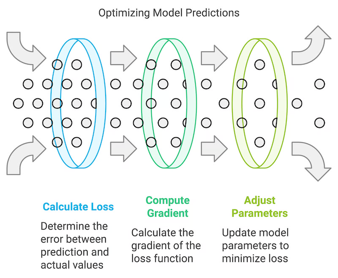
The real magic happens during the model.fit(...) call. What happens during the call for each epoch:

• The model iterates over train_ds
• For each batch:
  • makes predictions
  • computes loss
  • computes gradients
  • updates weights via the optimizer
• After an epoch, it evaluates on val_ds to measure generalization

With the submission of the validation_data we make sure not to overfit the model.

Analyse the training progress

This step is purly for your evaluation of the training progress. Let’s get an overview on whats good and whats bad:

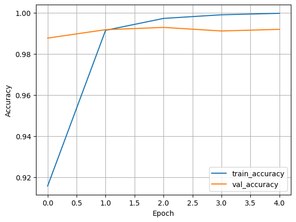
Accuracy

• train_accuracy describes how well the model fits the training data
• val_accuracy describes how well it generalizes to unseen data

Good sign: both curves rising and staying reasonably close

Overfitting sign: training goes up, validation gets worse or stagnates

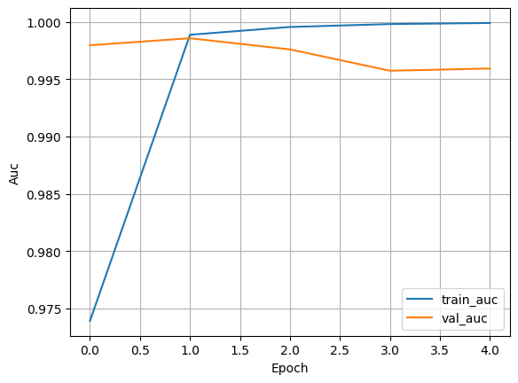
AUC

• Higher AUC describes the model is better at distinguishing spam vs ham
• AUC is especially useful when the classes are imbalanced

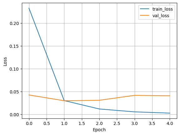
Loss

• train_loss should go down as the model learns
• val_loss ideally also decreases, then stabilizes

If the train_loss keeps decreasing and val_loss starts increasing after some epoch this would indicate a strong overfitting.

#@title Plot training curves

def plot_history(history, metric="accuracy"):
    plt.figure()
    plt.plot(history.history[metric], label=f"train_{metric}")
    plt.plot(history.history[f"val_{metric}"], label=f"val_{metric}")
    plt.xlabel("Epoch")
    plt.ylabel(metric.capitalize())
    plt.legend()
    plt.grid(True)
    plt.show()

plot_history(history, "accuracy")
plot_history(history, "auc")
plot_history(history, "loss")

Examples